Chapter 4 Somatic mutation analysis in single cells

Here is the runnable notebook 03-CellularGenetics-ntb.Rmd (download by right click and “Save Link As”)

4.1 Introduction

Whole genome (or exome) sequencing at bulk tissues have been widely used in studying somatic mutation in cancer samples and healthy tissues recently. It allows to identify somatic mutations and accurately estimate of the frequency of each mutation (see Fig. 4.1, adapted from Kuipers et al, 2017).

However, there are a few major challenges in somatic mutations with bulk sequencing.

• First, the allele frequency cannot give accurate clonal structure, as it is difficult to distinct mutations from different clones that have similar population percents.
• Second, the evolutionary lineage is much difficult to infer from bulk sequencing data without single cell resolution
• Third, the bulk DNA-seq cannot dissect the phenotypic impact of somatic mutations, which however is crucial to understand intra-tumor heterogeneity, both at genetic and transcriptomic levels.

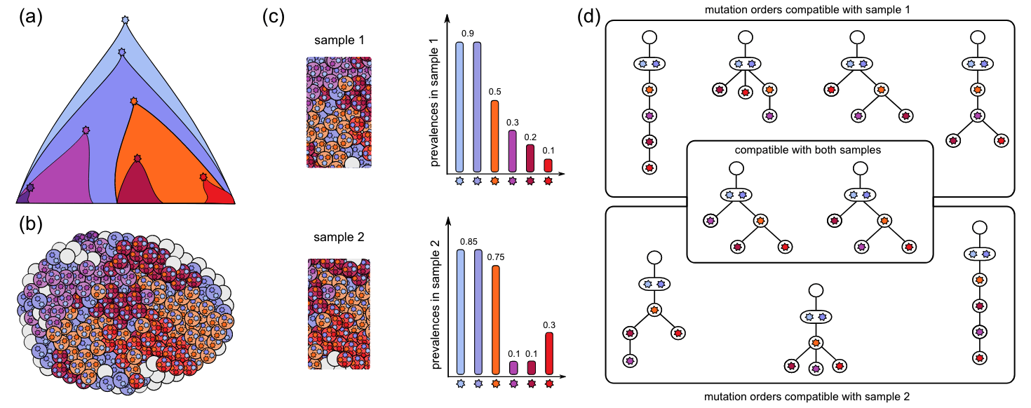
Figure 4.1. Somatic mutations and evolution. Fig adapted from Kuipers et al, 2017

4.1.1 Choice of protocols

Let’s first review the different protocols for single-cell sequencing, as genetic analysis often higher requirement of sequencing coverage.

In next Figure from Ding et al, 2020, there are major two different types of protocols. One is well based, including SMART-seq, returning moderate coverage but low number of cells. The other is droplet-based, including 10x Genomics, returning extremely low coverage but high number of cells.

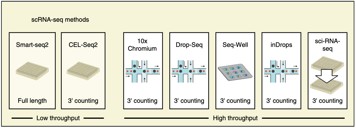
Figure 4.2. Common protocols of scRNA-seq. Fig adapted from Ding et al, 2020

Though scRNA-seq contains the information of somatic mutations in the expressed RNA molecules. However, it only covers the highly expressed genes (or its 3’ / 5’ if UMI-based protocols). Generally, scDNA-seq offers more even coverage across the genome, despite its much higher cost. Nonetheless, given the low capture efficiency, all protocols suffer from allele drop-out, namely false negatives in observing the existing mutation allele.

Below, we summarize different sequencing strategies and their potentials for analyzing different types of somatic mutations, including copy number variations (CNV), single-nucleotide variation (SNV) and mitochondrial SNV (mtSNV).

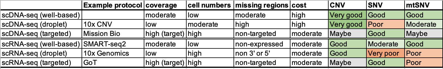
Table 4.1. Protocols for cellular genetic analysis

In the following sections, we will show two example data sets to illustrating:

• SMART-seq2 for SNV and mtSNV analysis
• 10x Genomic for CNV analysis (and possibly mtSNV analysis if lucky)

4.2 SNV analysis

Here, we will use a SMART-seq2 dataset, the joxm dataset (77 QC cells) generated from McCarthy et al, 2020), as an example of SNV analsyis in single cells (Fig. 4.3 below for this donor). The processed data sets are directly available from its according cardelino R package. We also prepared the raw data (in .bam format) and scripts to generate them in Chapter 6.2 for you to practice the preprocessing steps with tools cellsnp-lit and MQuad.

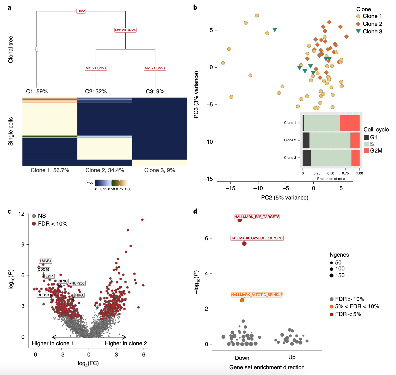
Figure 4.3. SNVs analysis with Joxm dataset. Fig adapted from McCarthy et al, 2020

4.2.1 Call somatic variants and genotype single cells

Nuclear genome is large and scRNA-seq is generally noisy, hence making it extremely difficult to call somatic SNVs from scRNA-seq data directly. In this dataset, probably in a general situation, we could detect somatic SNVs using bulk whole genome sequencing with tumor and matched normal samples first, e.g., with the commonly used MuTect.

In this joxm dataset, we have called ~650 SNVs from bulk whole exome-seq. Given this list of called somatic variants, we can genotype each cell with genotyping tool. Here, we used our cellsnp-lit (with high recommendation).

Finally, we obtained 112 SNVs are expressed in at least one of the 77 cells. The output file in VCF is available in the cardelino package cellSNP.cells.vcf.gz (12KB).

4.2.2 Visualize variat allele fequency

Now, let’s load the data and visualise the allele frequency here:

library(ggplot2)
library(cardelino)

vcf_file <- system.file("extdata", "cellSNP.cells.vcf.gz", package = "cardelino")
input_data <- load_cellSNP_vcf(vcf_file)

AF <- as.matrix(input_data$A / input_data$D)

p = pheatmap::pheatmap(AF, cluster_rows=FALSE, cluster_cols=FALSE,
                   show_rownames = TRUE, show_colnames = TRUE,
                   labels_row='77 cells', labels_col='112 SNVs',
                   angle_col=0, angle_row=0)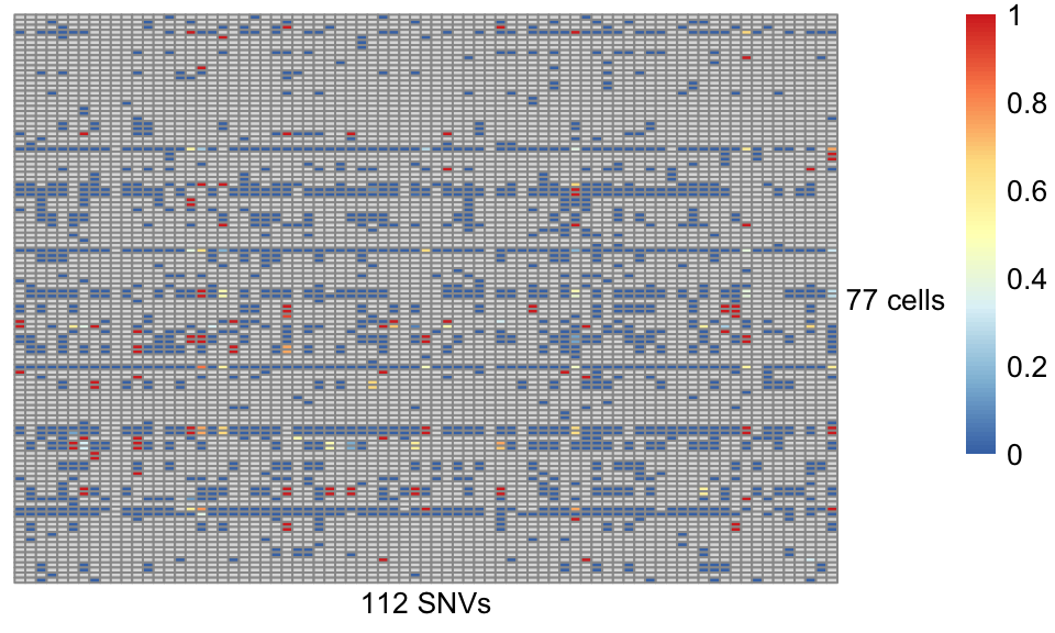

Figure 4.4. Allele frequency of somatic SNVs in Joxm dataset

As expected, the majority of entries are missing (in grey) due to the high sparsity in scRNA-seq data. For the same reason, even for the non-missing entries, the estimate of allele frequency is of high uncertainty. Therefore, it is crucial to probabilistic clustering with accounting the uncertainty, ideally with guide clonal tree structure from external data.

4.2.3 Use extra information on clonal tree

As mentioned, the variant calling is based on bulk WES, which can also be used to infer a clonal tree, even though it is of high uncertainty by only using bulk data. Here, we obtain a maximum-a-posteriori (MAP) tree from Canopy. The clonal tree inferred by Canopy for this donor consists of three clones, including a “base” clone (“clone1”) that has no clonal somatic mutations present.

canopy_res <- readRDS(system.file("extdata", "canopy_results.coveraged.rds", 
                                  package = "cardelino"))
plot_tree(canopy_res$tree, orient = "v")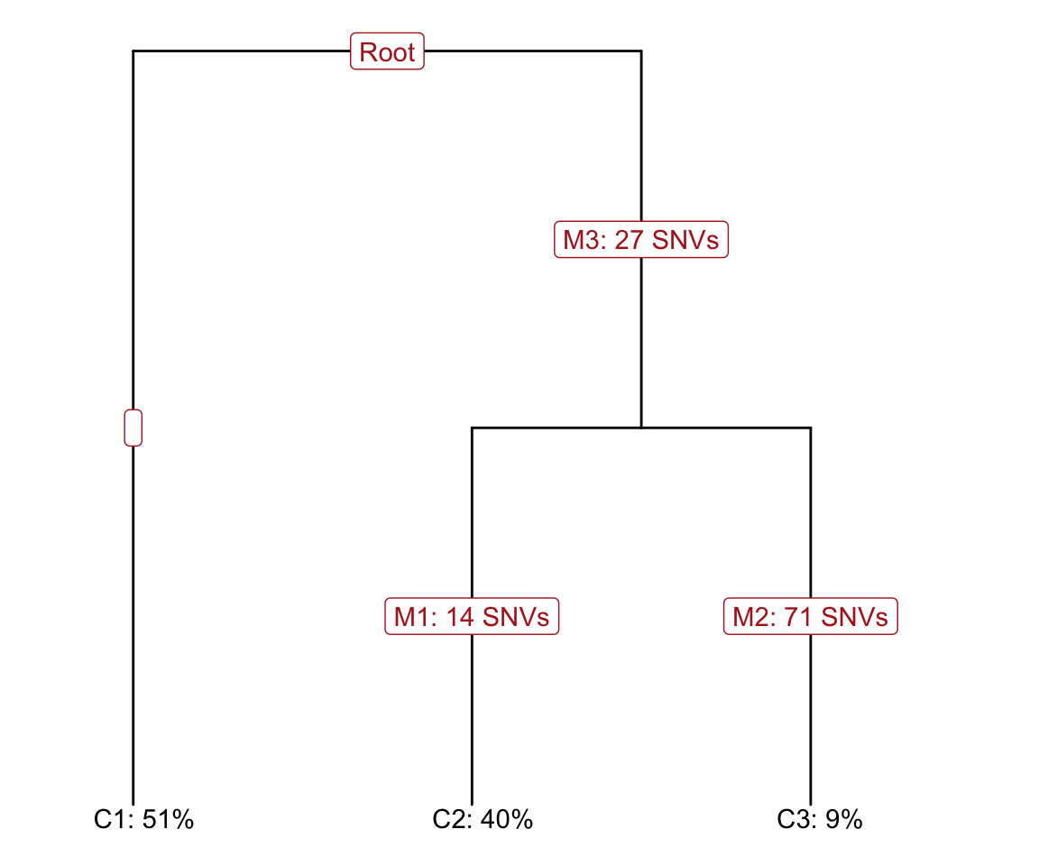

Figure 4.5. Clonal tree inferred from bulk WES data

4.2.4 Run cardelino for inferring clonal structure

Now, we can leverage the inferred clonal tree as an guidance to cluster cells based on their mutation profiles.

Before starting, be careful to ensure that the same variant IDs are used in both data sources.

Config <- canopy_res$tree$Z
rownames(Config) <- gsub(":", "_", rownames(Config))

The run clone_id the main function in cardelino package:

set.seed(7)
assignments <- clone_id(input_data$A, input_data$D, Config = Config,
                        min_iter = 800, max_iter = 1200)
names(assignments)

We can visualize the cell-clone assignment probabilities as a heatmap.

prob_heatmap(assignments$prob)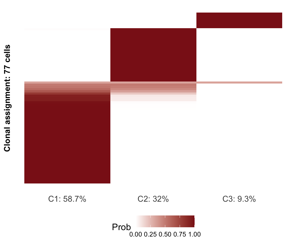

Figure 4.6. Assignment probability of cells to clones

We recommend assigning a cell to the highest-probability clone if the highest posterior probability is greater than 0.5 and leaving cells “unassigned” if they do not reach this threshold. The assign_cells_to_clones function conveniently assigns cells to clones based on a threshold and returns a data.frame with the cell-clone assignments.

df <- assign_cells_to_clones(assignments$prob)
head(df)
table(df$clone)

Also, Cardelino will update the guide clonal tree Config matrix (as a prior) and return a posterior estimate. In the figure below, negative value means the probability of a certain variant presents in a certain clone is reduced in posterior compared to prior (i.e., the input Config). Vice verse for the positive values.

heat_matrix(t(assignments$Config_prob - Config)) + 
  scale_fill_gradient2() +
  ggtitle('Changes of clonal Config') + 
  labs(x='Clones', y='112 SNVs') +
  theme(axis.text.y = element_blank(), legend.position = "right")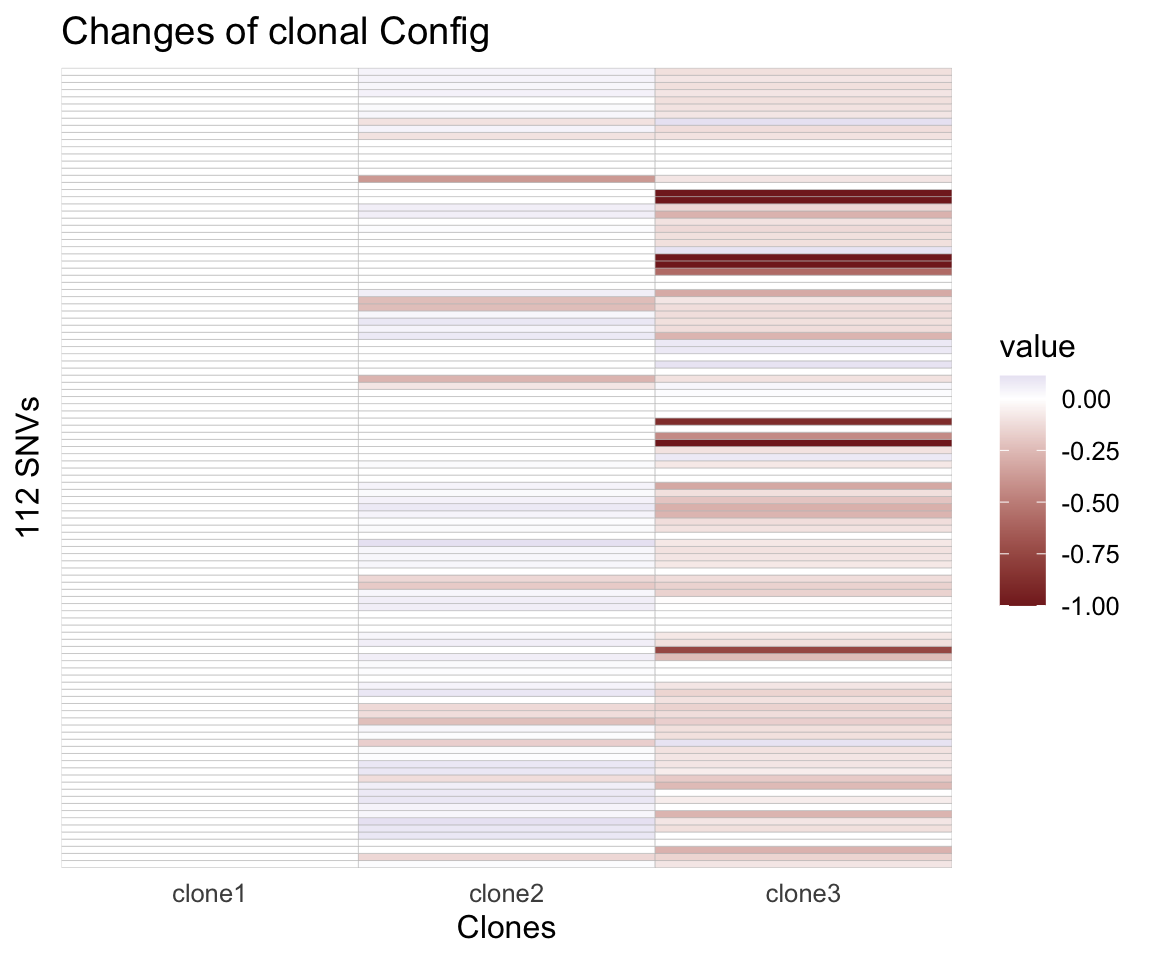

Figure 4.7. Difference between updated and input clonal configuration

Finally, we can visualize the results cell assignment and updated mutations clonal configuration at the raw allele frequency matrix:

AF <- as.matrix(input_data$A / input_data$D)
cardelino::vc_heatmap(AF, assignments$prob, Config, show_legend=TRUE)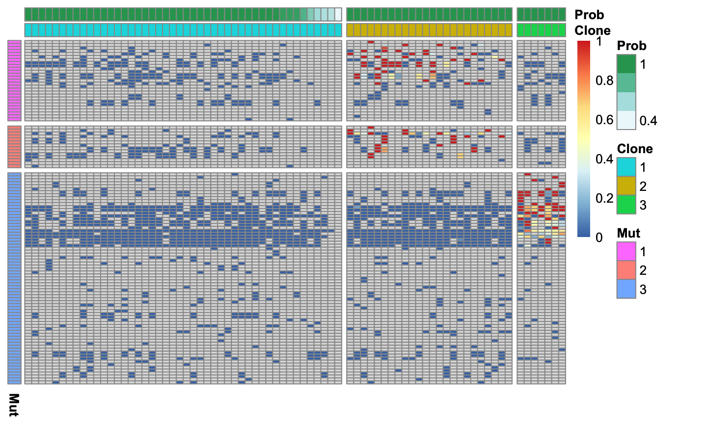

Figure 4.8. Allele frequency of clustered cells and variants

4.3 mtSNV analysis

Recently, mitochondrial variants have also been shown powerful makeups for lineage tracing Ludwig et al, 2019. The much higher copies of mtDNA not only give much higher sequencing coverage, but generally highly mutation rate (probably also some other biological reasons).

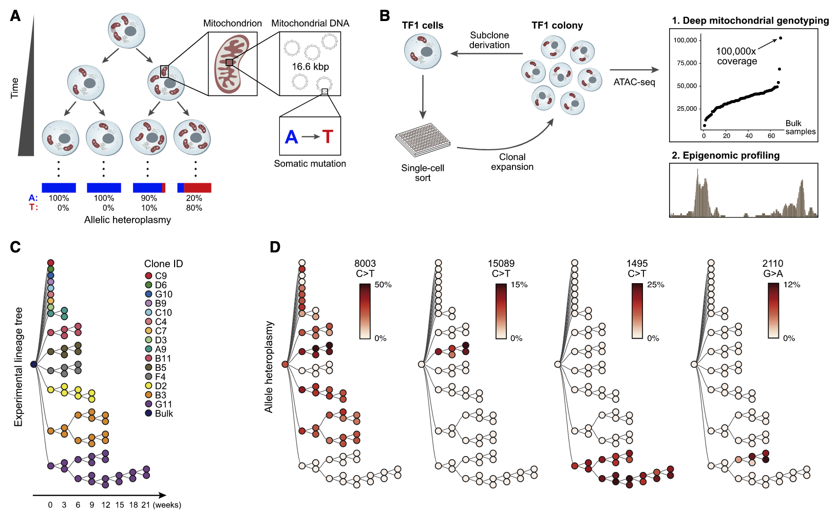
Figure 4.9. Mitochondrial variants for lineage tracing. Fig. adapted from Ludwig et al, 2019

4.3.1 Visualise allele frequency

Here, we illustrate the mtDNA on the joxm dataset again. During the preprocssing (see Chapter 7.2), we first genotype the whole mito genome directly with cellsnp-lit and then call the clonal informed variants by MQuad.

Let’s first load the processed dataset from cardelino package and visualize the allele frequency.

AD_file <- system.file("extdata", "passed_ad.mtx", package = "cardelino")
DP_file <- system.file("extdata", "passed_dp.mtx", package = "cardelino")
id_file <- system.file("extdata", "passed_variant_names.txt", package = "cardelino")

AD <- Matrix::readMM(AD_file)
DP <- Matrix::readMM(DP_file)
var_ids <- read.table(id_file, )
rownames(AD) <- rownames(DP) <- var_ids[, 1]
colnames(AD) <- colnames(DP) <- paste0('Cell', seq(ncol(DP)))

AF_mt <- as.matrix(AD / DP)
pheatmap::pheatmap(AF_mt)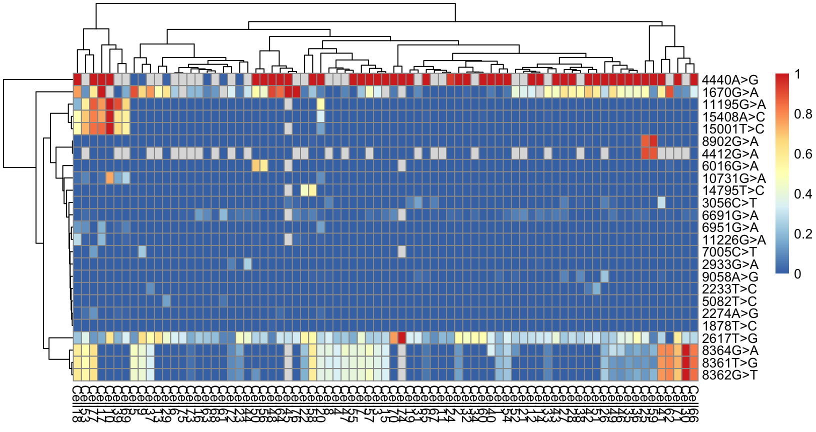

Figure 4.10. Allele frequency of mtDNA variants

As expected, the coverage of mtDNA is a lot higher than the nuclear genome above (much fewer missing values).

4.3.2 Infer clonal structure with mtDNA variants

Now, we can run cardelino on the mitochondrial variations. Note, as there is no prior clonal tree, the model is easier to return a local optima. Generally, we recommend running it multiple time (with different random seed or initialization) and pick the one with highest DIC.

set.seed(7)
assign_mtClones <- clone_id(AD, DP, Config=NULL, n_clone = 3, keep_base_clone=FALSE)

Then visualize allele frequency along with the clustering of cells and variants:

Config_mt <- assign_mtClones$Config_prob
Config_mt[Config_mt >= 0.5] = 1
Config_mt[Config_mt <  0.5] = 0
cardelino::vc_heatmap(AF_mt, assign_mtClones$prob, Config_mt, show_legend=TRUE)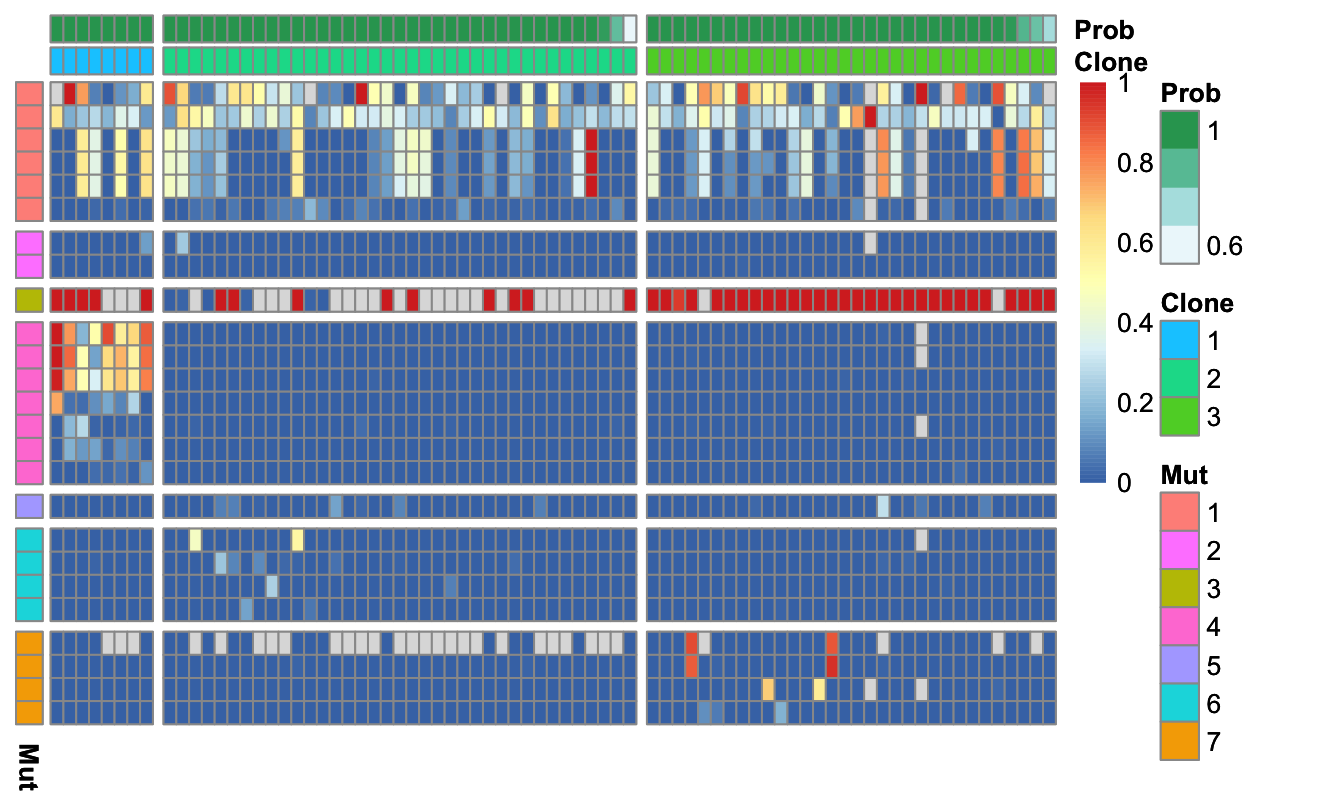

Figure 4.11. Allele frequency of mtSNVs with clustered cells

4.4 Last notes

As shown, cardelino allows us to cluster cells based on somatic mutations with accounting for the high uncertainty caused by technical variability. Last, we’d like to highlight a few potential drawbacks of cardelino:

1. It is computationally expensive due to the nature of Gibbs sampling that scarifies speed for accuracy. For large data sets, e.g., >1000 cells, cardelino may be too slow to handle. If speed is a major concertain, please consider our more efficient tool Vireo as a sister tool.

2. It may not always return a converged results. You could consider running it longer or with more chains or initialization.

3. It is generally difficult to select the best number of clone. You may get some clue by trial and error or visualise it from hierarchical clustering first.

Feel free to get in touch (yuanhua@hku.hk) if you need advice on somatic mutation analysis on your own data / project.