Chapter 5 Copy number variation estimation from scRNA-seq
5.1 Introduction
Copy number variation is a major mutations in many tumors. Recently, Minussi et al, 2021 suggested novel evolutionary patterns through analyzing CNV in breast tumors.
There are three types of CNVs:
- Copy gain
- Copy loss
- Loss of heterozygosity
They some may not affect the total copies, e.g., Loss of heterozygosity, while some may not affect the balance of two allele, e.g., copy gain (2 vs 2).
There are four major methods for CNV analyis in scRNA-seq:
Here, we will illustration how to use the method inferCNV for analysing CNV in
single-cell RNA-seq data. We will discuss other methods in the end.
5.2 inferCNV and example
InferCNV: Inferring copy number alterations from tumor single cell RNA-Seq data
5.2.1 install inferCNV
Software Requirements
- JAGS
- R (>3.6)
In order to run infercnv, JAGS (Just Another Gibbs Sampler) must be installed.
Download JAGS from https://sourceforge.net/projects/mcmc-jags/files/JAGS/4.x/ and install JAGS in your environment (windows/MAC).
If you use inferCNV on server, install JAGS via conda install in your conda environment is recommended.
conda install -c conda-forge jagsMore details refer to inferCNV wiki page
Five options for installing inferCNV
Option A: Install infercnv from BioConductor (preferred)
if (!requireNamespace("BiocManager", quietly = TRUE))
     install.packages("BiocManager")
BiocManager::install("infercnv")
For more other options, refer to Five options for installing inferCNV
Data requirements
- a raw counts matrix of single-cell RNA-Seq expression
- an annotations file which indicates which cells are tumor vs. normal.
- a gene/chromosome positions file
5.2.2 getting started
If you have installed infercnv from BioConductor, you can run the example data with:
library(infercnv)

infercnv_obj = CreateInfercnvObject(raw_counts_matrix=system.file("extdata", "oligodendroglioma_expression_downsampled.counts.matrix.gz", package = "infercnv"),
                                    annotations_file=system.file("extdata", "oligodendroglioma_annotations_downsampled.txt", package = "infercnv"),
                                    delim="\t",
                                    gene_order_file=system.file("extdata", "gencode_downsampled.EXAMPLE_ONLY_DONT_REUSE.txt", package = "infercnv"),
                                    ref_group_names=c("Microglia/Macrophage","Oligodendrocytes (non-malignant)"))

infercnv_obj = infercnv::run(infercnv_obj,
                             cutoff=1, # cutoff=1 works well for Smart-seq2, and cutoff=0.1 works well for 10x Genomics
                             out_dir=tempfile(),
                             cluster_by_groups=TRUE,
                             denoise=TRUE,
                             HMM=TRUE)
If you can run the getting started part with demo data provided by inferCNV, then it is installed successfully.
Demo Example Figure
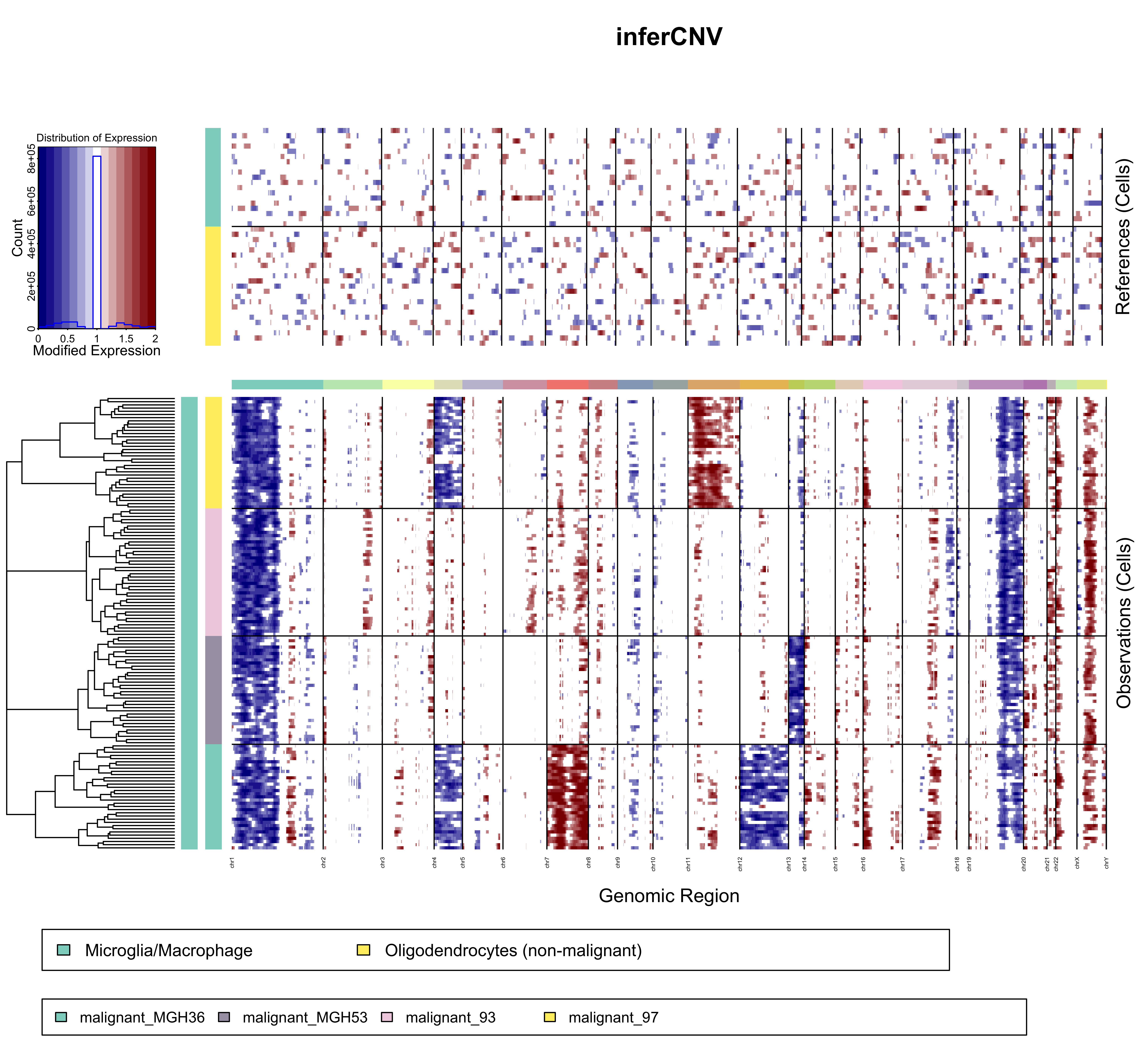
Demo Example Figure
5.3 Application on TNBC1
5.3.1 data description
TNBC1 is a triple negative breast cancer tumor sample of high tumor purity (72.6%) with 796 single tumor cells and 301 normal cells. The dataset is available on NCBI GEO under the accession number GSM4476486.
| TNBC1 | Number of clones | Number of tumor clones | Tumor clone-specific copy gain |
|---|---|---|---|
| Triple negative breast cancer | |
|
|
- Expression
| Clone A | Clone B | Normal |
|---|---|---|
| 488 | 307 | 302 |
Notes: 488,307, 247, 55
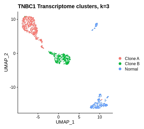
umap
- B Allele Frenquency (BAF)
baf1
baf2
baf3
- BAF V.S. Expression
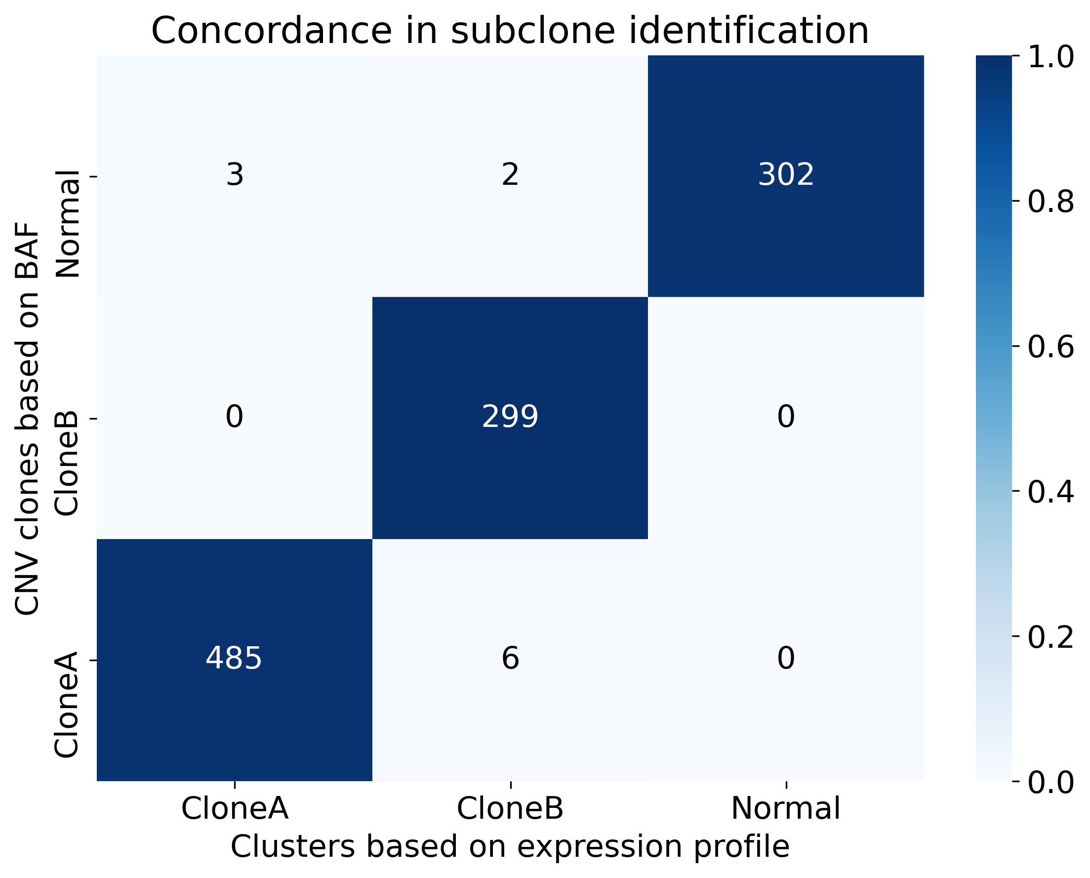
confusion heatmap
5.3.2 run inferCNV
# library(infercnv)
# library(utils)
# library (BiocGenerics)

## DEMO1
#
# tnbc <- read.delim("C://Users/Rongting/Documents/GitHub_repos/combinedTNBC1.txt")
# anno <- tnbc[2,]
# anno <- t(anno)
# anno <- as.data.frame(anno)
#
# gex <- tnbc[-c(1:2),]
# gex <- type.convert(gex)
#
# gene_file <- "C://Users/Rongting/Documents/GitHub_repos/gene_note_noheader_unique.txt"

#
# infercnv_obj = CreateInfercnvObject(raw_counts_matrix=gex,
#                                     annotations_file=anno,
#                                     delim='\t',
#                                     gene_order_file=gene_file,
#                                     ref_group_names= "N")

# output = "C://Users/Rongting/Documents/GitHub_repos/tnbc1_demo"

# infercnv_obj = infercnv::run(infercnv_obj,
#                              cutoff=0.1,
#                              out_dir= output ,
#                              cluster_by_groups=T,
#                              denoise=T,
#                              HMM=T)

## DEMO2

# gene_file <- "C://Users/Rongting/Documents/GitHub_repos/gene_note_noheader_unique.txt"
#
# anno_file <- 'C://Users/Rongting/Documents/GitHub_repos/tnbc-3cluster-id.txt'
#
# infercnv_obj2 = CreateInfercnvObject(raw_counts_matrix=gex,
#                                     annotations_file=anno_file,
#                                     delim='\t',
#                                     gene_order_file=gene_file,
#                                     ref_group_names= "Normal")
#
# output = "C://Users/Rongting/Documents/GitHub_repos/tnbc1_demo2"
#
# infercnv_obj2 = infercnv::run(infercnv_obj2,
#                              cutoff=0.1,
#                              out_dir= output,
#                              cluster_by_groups=T,
#                              denoise=T,
#                              HMM=T)
#################
##Notes
#################
## load the package
library(Seurat)
library(infercnv)
## prepare the data (cellranger output)
### load count matrix (example)
matrix_path <- "../cellranger/xxxx/count_xxxxx/outs/filtered_gene_bc_matrices/GRCh38/"
### read count matrix
gex_mtx <- Seurat::Read10X(data.dir = matrix_path)
### run inferCNV with loop
celltype = c('CloneA', 'CloneB', 'Normal')
for (i in celltype){
infercnv_obj1 = CreateInfercnvObject(raw_counts_matrix=gex_mtx,
annotations_file=anno_file,
delim='\t',
gene_order_file=gene_file,
ref_group_names=c(i))
output <- paste0('/groups/cgsd/rthuang/processed_data/inferCNV/xxxx/','xxxx_', i)
infercnv_obj1 = infercnv::run(infercnv_obj1,
cutoff=0.1,
out_dir= output ,
cluster_by_groups=T,
denoise=T,
HMM=T)
}
5.3.3 inferCNV result
- demo1
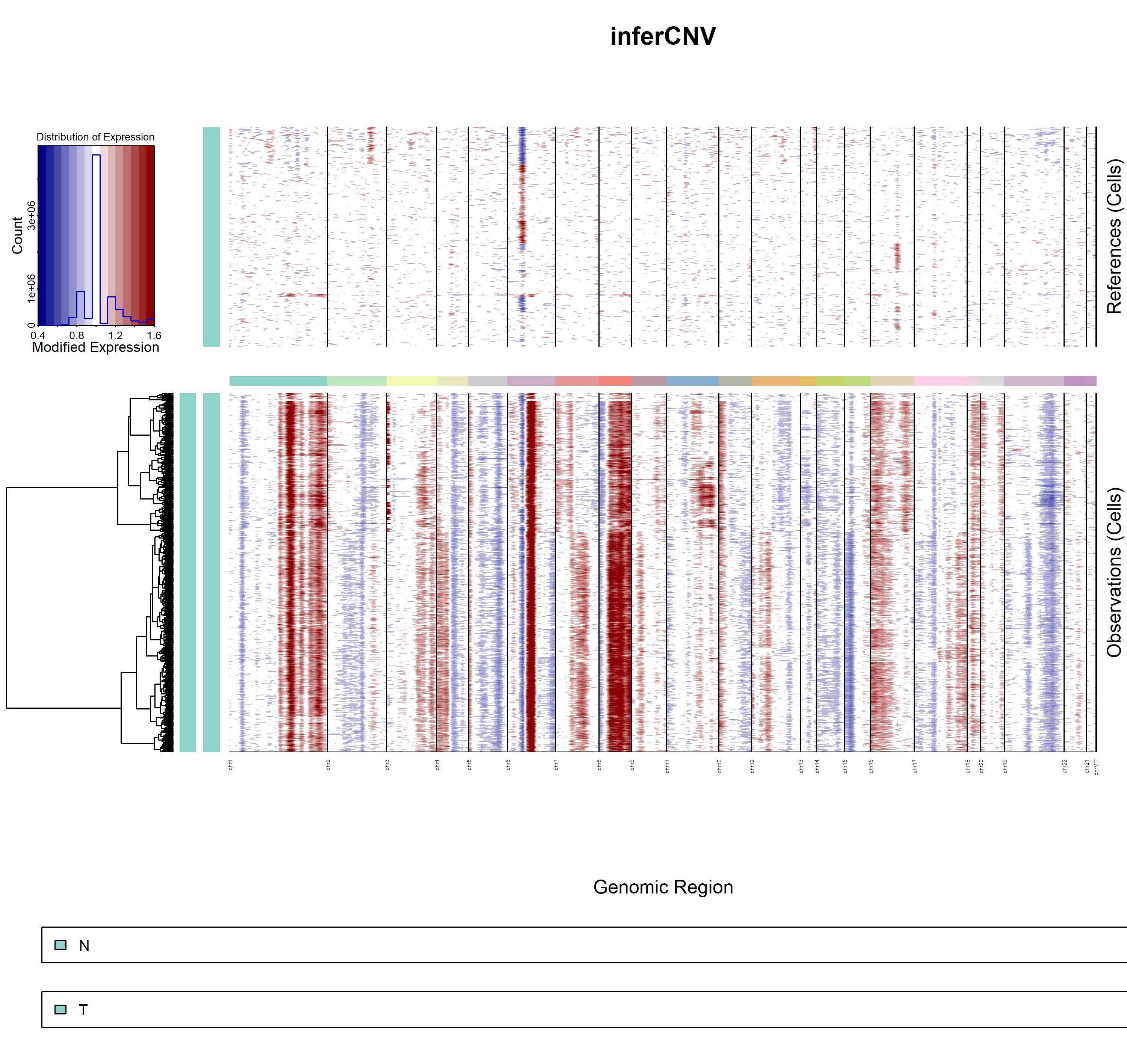
infercnv1
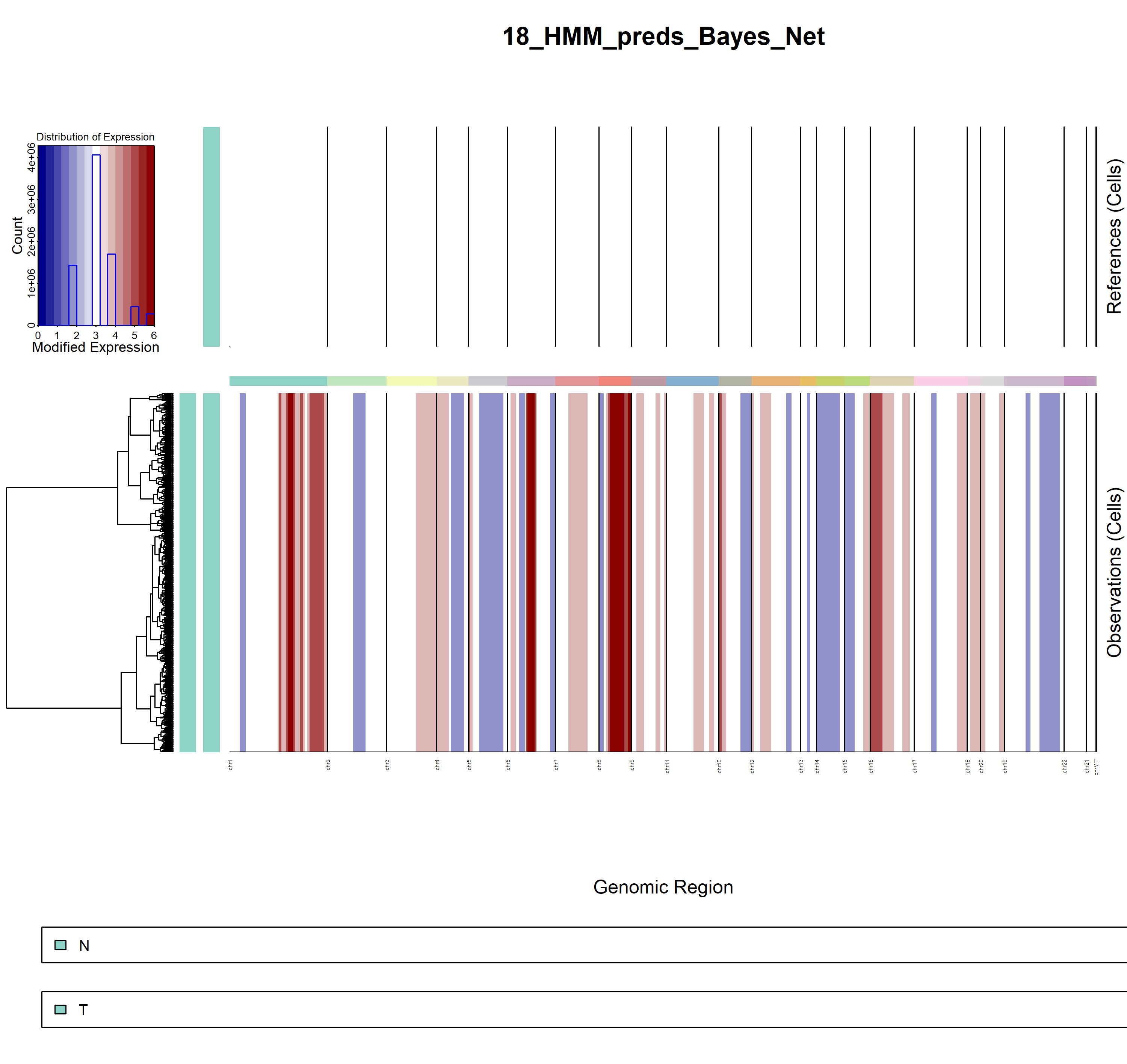
infercnv2
- demo2
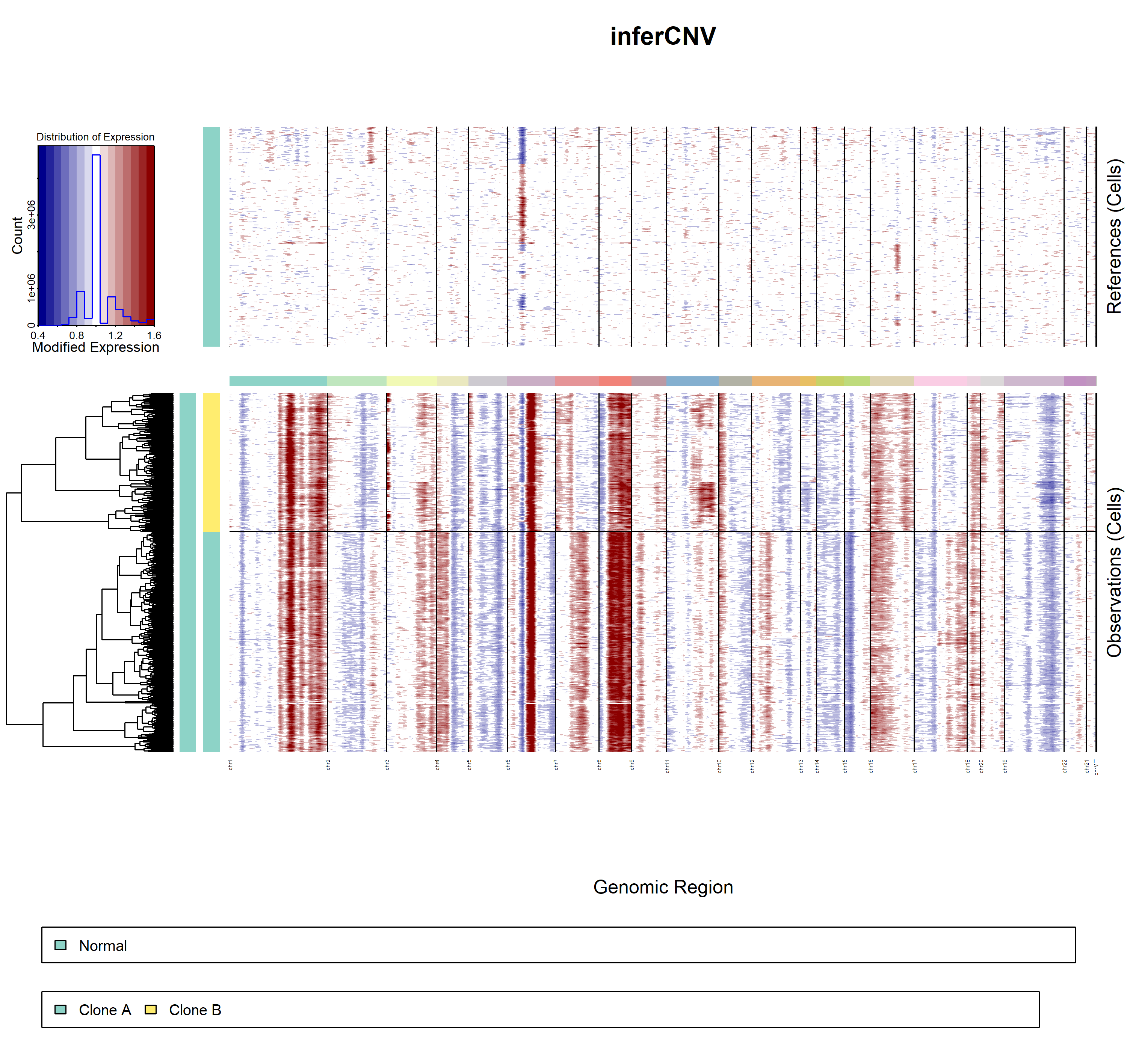
infercnv3
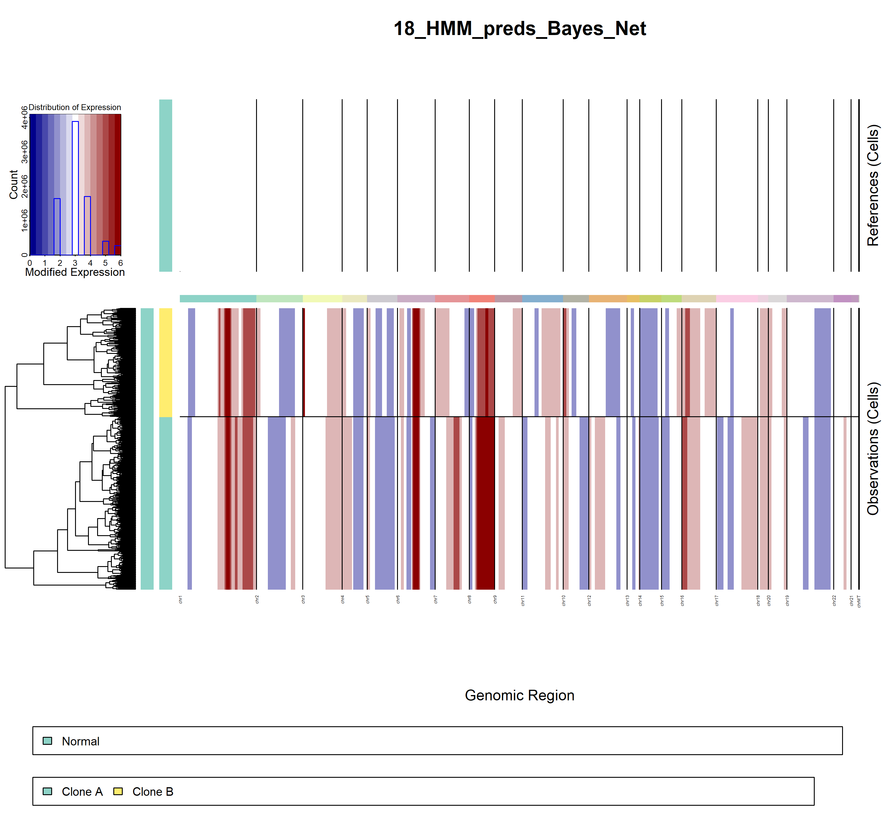
infercnv4
5.4 Last notes
There are four major methods for CNV analyis in scRNA-seq: inferCNV, CopyKat, CaSpER, and HoneyBadger
However, the two BAF-supporting methods HoneyBadger and Casper works less accurately from our experience. The expression-only method InferCNV and CopyKat generally works fine, though it has no capability to detect loss of heterozygosity. In general, we suggest perform a pseudo-bulk BAF on the identified clones or cell clusters with copy number variations.
Feel free to get in touch (yuanhua@hku.hk) if you need advice on CNV analysis on your own data / project.
ref
https://www.r-bloggers.com/2012/04/getting-started-with-jags-rjags-and-bayesian-modelling/
bookdown::render_book("index.Rmd", "bookdown::gitbook")