Chapter 7 Population Genetics and Diseases

7.1 Case study 1: Heritability and human traits

7.1.1 Part 1

Scenario: You are a researcher working on a twin study on cardiovascular traits to assess the genetic and environmental contribution relevant to metabolism and cardiovascular disease risk. You have recruited a cohort of volunteer adult twins of the same ancestry. The volunteers have undergone a series of baseline clinical evaluations and performed genotyping on a panel of single nucleotide polymorphisms that may be associated with the traits.

7.1.1.1 Questions for Discussion

Q1. Besides the clinical measurements, what data do you need to collect from the subjects?

Answers:

• Sex
• Age
• Other confounding factors, e.g. BMI, blood pressure, smoking status, etc.

Q2. How is genotype data represented for statistical genetic analysis?

Answers:

• Allele: 0/1, 1/2, A/C, etc
• Genotype: 0 0, 0 1, 1 0, 1 1
• Genotype probabilities: P(0/0)=0, P(0/1)=1, P(1/1)=0
• Genotype dosage: 0/1/2, 0.678 (continuous from 0-1 or 0-2)

Q3. How can you test for association between genotypes and phenotypes (binary and quantitative)?

Answers:

• Allelic chi-square test
• Fisher’s exact test
• Linear/Logistic regression
• Linear mixed model

7.1.1.2 Hands-on exercise : Association test

Now, you are given a dataset of age- and sex-matched twin cohort with two cardiovascular phenotypes and 5 quantitative trait loci (QTL). Data set and template notebook are available on Moodle (recommended) and also on this GitHub Repo.

The information for columns:

• zygosity: 1 for monozygotic (MZ) and 2 for dizygotic (DZ) twin
• T1QTL_A[1-5] and T2QTL_A[1-5]: 5 quantitative loci (A1-A5) in additive coding for Twin 1 (T1) and Twin 2 (T2) respectively
• The same 5 QTL (D1-D5) in dominance coding for T1 and T2
• Phenotype scores of T1 and T2 for the two quantitative cardiovascular traits

Download the data dataTwin2024.dat to your working directory. Start the RStudio program and set the working directory.

dataTwin <- read.table("dataTwin2024.dat",h=T)

Exploratory analysis

Q1. How many MZ and DZ volunteers are there?

Answers:

• 1000 MZ and 1000 DZ

Q2. How are the genotypes represented?

Answers:

• Dosage/Count of non-reference allele : 0, 1, and 2
  • A1-5: The QTLs are biallelic with two alleles A and a. The genotypes aa, Aa, and AA are coded additively as 0 (aa), 1 (Aa) and 2 (AA).
  • D1-5: The genotypes aa, Aa, and AA are coded as 0 (aa), 1 (Aa) and 0 (AA).

Q3. Are the QTL independent of each other?

Answers:

• Yes. The pairwise correlations are low (<0.2).

Q4. Are there outliers in phenotypes?

Answers:

• Yes. T2 individual 1303 has phenotype score (-4.21) being 4 SD below the mean.

table(dataTwin$zygosity)        # Q1: shows number of MZ and DZ twin pairs
#> 
#>    1    2 
#> 1000 1000
table(dataTwin$T1QTL_A1)        # Q2: shows the distribution of QTL_A1
#> 
#>    0    1    2 
#>  474 1021  505
table(dataTwin$T1QTL_D1)        # Q2: shows the distribution of QTL_D1
#> 
#>    0    1 
#>  979 1021
table(dataTwin$T1QTL_A1, dataTwin$T1QTL_D1)     # Q2: shows the distribution of QTL_A1 in relation to QTL_D1
#>    
#>        0    1
#>   0  474    0
#>   1    0 1021
#>   2  505    0
cor(dataTwin[,2:11])                            # Q3: shows the correlation between QTL_As
#>             T1QTL_A1     T1QTL_A2     T1QTL_A3    T1QTL_A4     T1QTL_A5
#> T1QTL_A1  1.00000000 -0.005470340  0.021705688  0.01940408  0.016278190
#> T1QTL_A2 -0.00547034  1.000000000  0.017344822 -0.01421677 -0.008678746
#> T1QTL_A3  0.02170569  0.017344822  1.000000000  0.01335711 -0.036751338
#> T1QTL_A4  0.01940408 -0.014216767  0.013357109  1.00000000  0.074899996
#> T1QTL_A5  0.01627819 -0.008678746 -0.036751338  0.07490000  1.000000000
#> T2QTL_A1  0.53243815  0.004201635 -0.013909013  0.03252724  0.020081970
#> T2QTL_A2 -0.04561174  0.464131160 -0.005044127  0.01324172 -0.003012277
#> T2QTL_A3  0.03316574 -0.003552831  0.521253656  0.02045423  0.009081830
#> T2QTL_A4  0.03271254 -0.033419904  0.020422583  0.48641289  0.019247531
#> T2QTL_A5 -0.01285323  0.030413269 -0.045121964  0.08288145  0.457962222
#>              T2QTL_A1     T2QTL_A2     T2QTL_A3     T2QTL_A4    T2QTL_A5
#> T1QTL_A1  0.532438150 -0.045611740  0.033165736  0.032712539 -0.01285323
#> T1QTL_A2  0.004201635  0.464131160 -0.003552831 -0.033419904  0.03041327
#> T1QTL_A3 -0.013909013 -0.005044127  0.521253656  0.020422583 -0.04512196
#> T1QTL_A4  0.032527239  0.013241725  0.020454234  0.486412895  0.08288145
#> T1QTL_A5  0.020081970 -0.003012277  0.009081830  0.019247531  0.45796222
#> T2QTL_A1  1.000000000  0.006179257 -0.013129314  0.048294183 -0.01325839
#> T2QTL_A2  0.006179257  1.000000000 -0.020860987  0.002164782 -0.01131418
#> T2QTL_A3 -0.013129314 -0.020860987  1.000000000 -0.010583797 -0.02101270
#> T2QTL_A4  0.048294183  0.002164782 -0.010583797  1.000000000  0.04350925
#> T2QTL_A5 -0.013258394 -0.011314179 -0.021012699  0.043509251  1.00000000
cor(dataTwin[,2:11])>0.2
#>          T1QTL_A1 T1QTL_A2 T1QTL_A3 T1QTL_A4 T1QTL_A5 T2QTL_A1 T2QTL_A2
#> T1QTL_A1     TRUE    FALSE    FALSE    FALSE    FALSE     TRUE    FALSE
#> T1QTL_A2    FALSE     TRUE    FALSE    FALSE    FALSE    FALSE     TRUE
#> T1QTL_A3    FALSE    FALSE     TRUE    FALSE    FALSE    FALSE    FALSE
#> T1QTL_A4    FALSE    FALSE    FALSE     TRUE    FALSE    FALSE    FALSE
#> T1QTL_A5    FALSE    FALSE    FALSE    FALSE     TRUE    FALSE    FALSE
#> T2QTL_A1     TRUE    FALSE    FALSE    FALSE    FALSE     TRUE    FALSE
#> T2QTL_A2    FALSE     TRUE    FALSE    FALSE    FALSE    FALSE     TRUE
#> T2QTL_A3    FALSE    FALSE     TRUE    FALSE    FALSE    FALSE    FALSE
#> T2QTL_A4    FALSE    FALSE    FALSE     TRUE    FALSE    FALSE    FALSE
#> T2QTL_A5    FALSE    FALSE    FALSE    FALSE     TRUE    FALSE    FALSE
#>          T2QTL_A3 T2QTL_A4 T2QTL_A5
#> T1QTL_A1    FALSE    FALSE    FALSE
#> T1QTL_A2    FALSE    FALSE    FALSE
#> T1QTL_A3     TRUE    FALSE    FALSE
#> T1QTL_A4    FALSE     TRUE    FALSE
#> T1QTL_A5    FALSE    FALSE     TRUE
#> T2QTL_A1    FALSE    FALSE    FALSE
#> T2QTL_A2    FALSE    FALSE    FALSE
#> T2QTL_A3     TRUE    FALSE    FALSE
#> T2QTL_A4    FALSE     TRUE    FALSE
#> T2QTL_A5    FALSE    FALSE     TRUE
apply(dataTwin[22:25],2,function(x){ any(x < (mean(x) - 4*sd(x))) })  # Q4: any outlier < 4 SD from the mean for the two quantitative phenotypes
#> pheno1_T1 pheno1_T2 pheno2_T1 pheno2_T2 
#>     FALSE     FALSE     FALSE      TRUE
apply(dataTwin[22:25],2,function(x){ any(x > (mean(x) + 4*sd(x))) })  # Q4: any outlier > 4 SD from the mean for the two quantitative phenotypes
#> pheno1_T1 pheno1_T2 pheno2_T1 pheno2_T2 
#>     FALSE     FALSE     FALSE     FALSE
# remove the phenotype score of the outlier (T2) for the phenotype 2 (pheno2_T2)
outlier<- which(dataTwin$pheno2_T2 < (mean(dataTwin$pheno2_T2) - 4*sd(dataTwin$pheno2_T2) )) 
outlier
#> [1] 1303
dataTwin$pheno2_T2[outlier]
#> [1] -4.21
dataTwin$pheno2_T2[outlier] <- NA

Association test

Test for association between QTL and pheno1 for T1

• Regress pheno1_T1 on T1QTL_A1 to estimate the proportion of variance explained (R2).
• Model: pheno1_T1 = b0 + b1* T1QTL_A1 + e
• Calculate the conditional mean of phenotype (i.e. phenotypic mean conditional genotype)

If the relationship between the QTL and the phenotype is perfectly linear, the regression line should pass through the conditional means (c_means), and the differences between the conditional means should be about equal.

Q5. What are the values of b0, b1? Is QTL1 significant associated with the phenotype at alpha<0.01 (multiple testing of 5 loci)?

Answers:

• b0 = 4.1464
• b1 = 0.9180
• QTL1 is significantly associated with the phenotype with \(P = 1.02\times 10^{-13}\)

Q6. What is the proportion of phenotypic variance explained?

Answers:

• Proportion of phenotypic variance explained = 0.027

linA1 <- lm(pheno1_T1~T1QTL_A1, data=dataTwin)
summary(linA1)
#> 
#> Call:
#> lm(formula = pheno1_T1 ~ T1QTL_A1, data = dataTwin)
#> 
#> Residuals:
#>      Min       1Q   Median       3Q      Max 
#> -15.1225  -2.4435   0.1105   2.7775  12.2555 
#> 
#> Coefficients:
#>             Estimate Std. Error t value Pr(>|t|)    
#> (Intercept)   4.1464     0.1511  27.438  < 2e-16 ***
#> T1QTL_A1      0.9180     0.1226   7.491 1.02e-13 ***
#> ---
#> Signif. codes:  0 '***' 0.001 '**' 0.01 '*' 0.05 '.' 0.1 ' ' 1
#> 
#> Residual standard error: 3.834 on 1998 degrees of freedom
#> Multiple R-squared:  0.02732,    Adjusted R-squared:  0.02683 
#> F-statistic: 56.11 on 1 and 1998 DF,  p-value: 1.022e-13
summary(linA1)$r.squared  # proportion of explained variance by additive component
#> [1] 0.02731675

c_means <- by(dataTwin$pheno1_T1,dataTwin$T1QTL_A1,mean)
plot(dataTwin$pheno1_T1 ~ dataTwin$T1QTL_A1, col='grey', ylim=c(3,7))
lines(c(0,1,2), c_means, type="p", col=6, lwd=8)
lines(sort(dataTwin$T1QTL_A1),sort(linA1$fitted.values), type='b', col="dark green", lwd=3)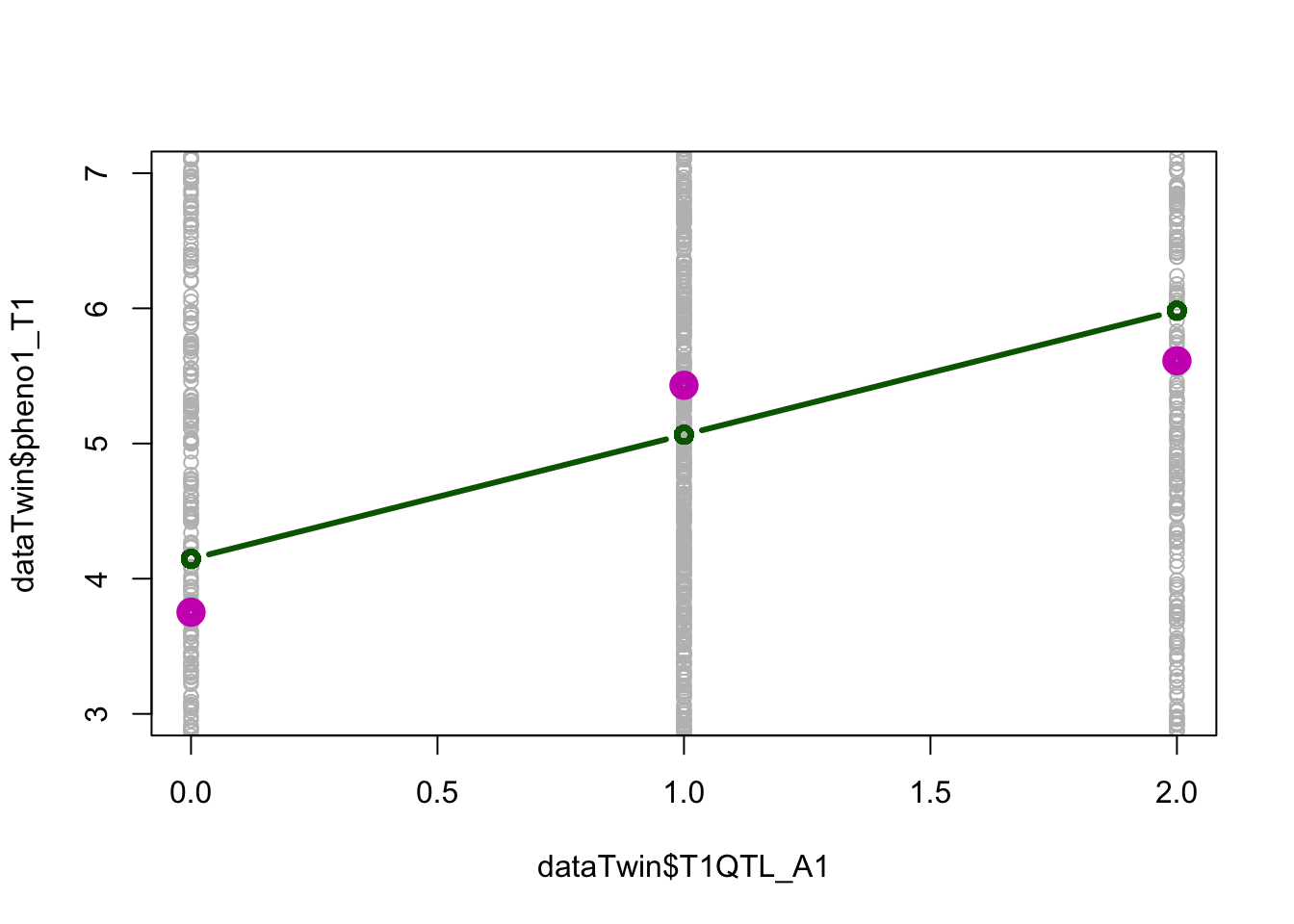

To test for the non-linearity, we can use the dominance coding of the QTL and add the dominance term to the regression model.

• Model: pheno1_T1 = b0 + b1* T1QTL_A1 + b2* T1QTL_D1 + e
• Repeat for T2.

Q7. Why can’t we analyse T1 and T2 together?

Answers:

• As T1 and T2 are biologically related as MZ or DZ twins, the genotypes of the QTLs are not independent. Treating the genotypes of T1 and T2 as independent observations will introduce bias.

Q8. Is there a dominance effect?

Answers:

• Yes. The model with dominance provides a better goodness of fit (lower p-value)

linAD1 <- lm(pheno1_T1 ~ T1QTL_A1 + T1QTL_D1, data=dataTwin)
summary(linAD1) # results lm(phenoT1~T1QTL_A1+T1QTL_D1)
#> 
#> Call:
#> lm(formula = pheno1_T1 ~ T1QTL_A1 + T1QTL_D1, data = dataTwin)
#> 
#> Residuals:
#>      Min       1Q   Median       3Q      Max 
#> -14.7524  -2.5131   0.0586   2.8215  11.8894 
#> 
#> Coefficients:
#>             Estimate Std. Error t value Pr(>|t|)    
#> (Intercept)   3.7522     0.1753  21.405  < 2e-16 ***
#> T1QTL_A1      0.9301     0.1220   7.622 3.83e-14 ***
#> T1QTL_D1      0.7483     0.1708   4.382 1.24e-05 ***
#> ---
#> Signif. codes:  0 '***' 0.001 '**' 0.01 '*' 0.05 '.' 0.1 ' ' 1
#> 
#> Residual standard error: 3.816 on 1997 degrees of freedom
#> Multiple R-squared:  0.03658,    Adjusted R-squared:  0.03562 
#> F-statistic: 37.91 on 2 and 1997 DF,  p-value: < 2.2e-16

plot(dataTwin$pheno1_T1 ~ dataTwin$T1QTL_A1, col='grey', ylim=c(3,7))
abline(linA1, lwd=3)
lines(c(0,1,2), c_means, type='p', col=6, lwd=8)
lines(sort(dataTwin$T1QTL_A1),sort(linA1$fitted.values), type='b', col="dark green", lwd=3)
lines(sort(dataTwin$T1QTL_A1),sort(linAD1$fitted.values), type='b', col="blue", lwd=3)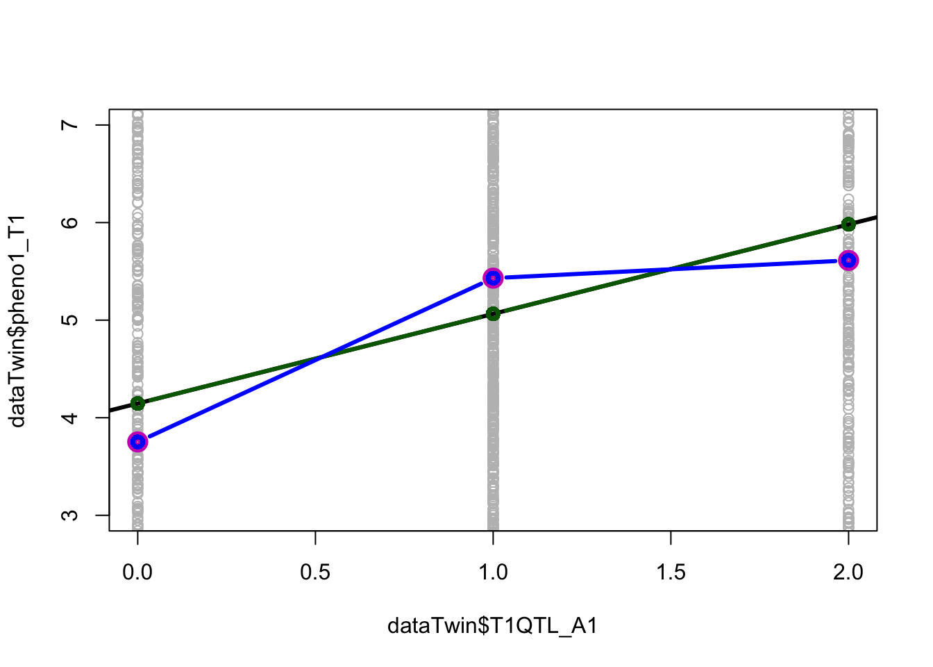

Q9. Repeat for the other 4 QTL and determine which QTL shows strongest association with the phenotype T1

Answers:

• QTL3 with \(P = 7.77 \times 10^{-25}\) for model with dominance

allQTL_A_T1 <- 2:6
cpheno1_T1 <- which(colnames(dataTwin)=="pheno1_T1")
## Additive
cbind(lapply(allQTL_A_T1,function(x){ fstat<- summary(lm(pheno1_T1 ~ ., data=dataTwin[,c(x,cpheno1_T1)]))$fstatistic;  pf(fstat[1],fstat[2],fstat[3],lower.tail = F) }))
#>      [,1]        
#> [1,] 1.021942e-13
#> [2,] 8.329416e-15
#> [3,] 1.007527e-13
#> [4,] 4.523758e-18
#> [5,] 8.207842e-13
## Dominance
cbind(lapply(allQTL_A_T1,function(x){ fstat<- summary(lm(pheno1_T1 ~ ., data=dataTwin[,c(x,x+10,cpheno1_T1)]))$fstatistic;  pf(fstat[1],fstat[2],fstat[3],lower.tail = F) }))
#>      [,1]        
#> [1,] 6.907834e-17
#> [2,] 2.166957e-22
#> [3,] 7.771588e-25
#> [4,] 8.124437e-25
#> [5,] 4.312127e-21

#Q9: QTL3 shows the strongest association with P=7.771588e-25
linAD3 <- lm(pheno1_T1 ~ T1QTL_A3 + T1QTL_D3, data=dataTwin)
summary(linAD3) # results lm(phenoT1~T1QTL_A1+T1QTL_D1)
#> 
#> Call:
#> lm(formula = pheno1_T1 ~ T1QTL_A3 + T1QTL_D3, data = dataTwin)
#> 
#> Residuals:
#>      Min       1Q   Median       3Q      Max 
#> -14.4988  -2.5701   0.1843   2.6991  11.5974 
#> 
#> Coefficients:
#>             Estimate Std. Error t value Pr(>|t|)    
#> (Intercept)   3.5437     0.1684  21.038  < 2e-16 ***
#> T1QTL_A3      0.9076     0.1181   7.683 2.43e-14 ***
#> T1QTL_D3      1.2714     0.1692   7.515 8.55e-14 ***
#> ---
#> Signif. codes:  0 '***' 0.001 '**' 0.01 '*' 0.05 '.' 0.1 ' ' 1
#> 
#> Residual standard error: 3.782 on 1997 degrees of freedom
#> Multiple R-squared:  0.05408,    Adjusted R-squared:  0.05313 
#> F-statistic: 57.09 on 2 and 1997 DF,  p-value: < 2.2e-16

If the subjects with top 10% of the phenotype score are considered as cases, perform case-control association test for most significant SNP (from Q9) and interpret the result.

Q10. What are the odds ratio, p-value, and 95% confidence interval (CI)?

Answers:

• Odds ratio is 4.28 and the 95% CI is (2.54, 7.20)

quant10 <- quantile(c(dataTwin$pheno1_T1),seq(0,1,0.1))
dataTwin$CaseT1 <- as.numeric(dataTwin$pheno1_T1>quant10[10])

dataTwin$T1QTL_AD3 <- (dataTwin$T1QTL_A3 + dataTwin$T1QTL_D3)/2

logisticAD3 <- summary(glm(CaseT1 ~ T1QTL_AD3, data=dataTwin, family="binomial"))
exp(logisticAD3$coefficients[2,1])                                     # odds ratio
#> [1] 4.277439
exp(logisticAD3$coefficients[2,1]-1.96*logisticAD3$coefficients[2,2])  # lower 95% confidence interval
#> [1] 2.539663
exp(logisticAD3$coefficients[2,1]+1.96*logisticAD3$coefficients[2,2])  # upper 95% confidence interval
#> [1] 7.204297

7.1.2 Part 2

Scenario: You are asked to estimate the additive genetic variance, dominance genetic variance and/or shared environmental variance using regression-based method and a classical twin design.

\[\begin{align*} \text{For ADE model : }~ & \sigma^{2}_{P} = \sigma^{2}_{A} + \sigma^{2}_{D} + \sigma^{2}_{E}\\ \text{For ACE model : }~ & \sigma^{2}_{P} = \sigma^{2}_{A} + \sigma^{2}_{C} + \sigma^{2}_{E}, \quad \text{where} \\ \sigma^{2}_{P} & \text{ is the phenotypic variance}, \\ \sigma^{2}_{A} & \text{ is additive genetic variance}, \\ \sigma^{2}_{D} & \text{ is dominance genetic variance}, \\ \sigma^{2}_{C} & \text{ is shared environmental variance, and} \\ \sigma^{2}_{E} & \text{ is unshared environmental variance.} \end{align*}\]

For ADE model, given the standardization of the phenotype,

\[\begin{align*} cov(MZ) = cor(MZ) & = rMZ = \sigma^{2}_{A} + \sigma^{2}_{D} \\ cov(DZ) = cor(DZ) & = rDZ = 0.5 * \sigma^{2}_{A} + 0.25 * \sigma^{2}_{D} \quad \text{ , where} \\ \end{align*}\] the coefficients 1/2 and 1/4 are based on quantitative genetic theory (Mather & Jinks, 1971).

By solving the unknowns, the variance explained by different components for the ADE model:

\[\begin{align*} \sigma^{2}_{A} & = 4*rDZ - rMZ \\ \sigma^{2}_{D} & = 2*rMZ - 4*rDZ \\ \sigma^{2}_{E} & = 1 - \sigma^{2}_{A} - \sigma^{2}_{D} \\ \end{align*}\]

For ACE model,

\[\begin{align*} cov(MZ) = cor(MZ) & = rMZ= \sigma^{2}_{A} + \sigma^{2}_{C} \\ cov(DZ) = cor(DZ) & = rDZ = 0.5 * \sigma^{2}_{A} + \sigma^{2}_{C} \quad \text{ , where} \\ \end{align*}\]

By solving the unknowns, the variance explained by different components for the ACE model:

\[\begin{align*} \sigma^{2}_{A} & = 2*(rMZ - rDZ) \\ \sigma^{2}_{C} & = 2*rDZ - rMZ \\ \sigma^{2}_{E} & = 1 - \sigma^{2}_{A} - \sigma^{2}_{C} = 1 - rMZ \end{align*}\]

7.1.2.1 Hands-on exercise : variance explained using regression-based method

Q1. What is the variance of the phenotype?

Q2. Compute the explained variance attributable to the additive genetic component of the QTL with strongest association in Part 1.

Q3. Compute the explained variance attributable to the dominance genetic component of the QTL with strongest association in Part 1.

R2 from the regression represents the proportion of phenotypic variance explained; thus the raw explained variance component is R2 times the variance of the phenotype (var_pheno).

Answers

• The proportion of explained variance are 0.0273 (additive) and 0.0541 (total: additive + dominance).
• As the predictors are uncorrelated, the proportion of explained variance by dominance = 0.0541 - 0.0273 = 0.0267
• Given the phenotypic variance of 15.102, then
  • Total genetic: 0.0541*15.102 = 0.8168
  • Additive genetic: 0.0273*15.102 = 0.4128
  • Dominance genetic: 0.0267*15.102 = 0.4040

var_pheno <- var(dataTwin$pheno1_T1)  # the variance of the phenotype
var_pheno
#> [1] 15.10257

linAD3 <- lm(pheno1_T1 ~ T1QTL_A3 + T1QTL_D3, data=dataTwin)
linA3 <- lm(pheno1_T1 ~ T1QTL_A3, data=dataTwin)

summary(linAD3)$r.squared           # proportion of explained variance by total genetic component
#> [1] 0.05408025
summary(linA3)$r.squared            # proportion of explained variance by additive component
#> [1] 0.02733034
summary(linAD3)$r.squared*var_pheno # (raw) variance component of total genetic component
#> [1] 0.8167509
summary(linA3)$r.squared*var_pheno  # (raw) variance component of additive genetic component
#> [1] 0.4127585
(summary(linAD3)$r.squared-summary(linA3)$r.squared)*var_pheno  # (raw) variance component of dominance genetic component
#> [1] 0.4039924

Q4. Estimate the variance explained by all the QTL using linear regression.

Answers

• Proportion of variance explained by all 5 QTLs with dominance = 0.23 and the total variance explained = 3.52.

# compute for all 5 QTL
linAD5=(lm(pheno1_T1 ~ T1QTL_A1 + T1QTL_A2 + T1QTL_A3 + T1QTL_A4 + T1QTL_A5 +
                       T1QTL_D1 + T1QTL_D2 + T1QTL_D3 + T1QTL_D4 + T1QTL_D5,
            data=dataTwin))

summary(linAD5)$r.squared              # proportion of explained variance by total genetic component
#> [1] 0.2330307
summary(linAD5)$r.squared*var_pheno    # (raw) variance component of total genetic component
#> [1] 3.519363

7.1.2.2 Hands-on exercise : variance explained using a classical twin design.

Based on our regression results, we have estimates of the total genetic variance as well as the A and D components for phenotype 1 explained by the QTLs. In practice, it is impossible to know all the variants associated with any polygenic trait.

Alternatively, we can use ADE or ACE models to estimate the A (additive genetic) and D (dominance)/C (shared environmental) variance with the classical twin design for phenotype 1 without genotypes.

Q5. Which model should be used? ACE or ADE? Let’s first compute rMZ and rDZ.

Answers

• rMZ = 0.5434
• rDZ = 0.1904
• As \(rMZ > 2*rDZ\), ADE model should be used.

dataMZ = dataTwin[dataTwin$zygosity==1, c('pheno1_T1', 'pheno1_T2')] # MZ data frame
dataDZ = dataTwin[dataTwin$zygosity==2, c('pheno1_T1', 'pheno1_T2')] # DZ data frame

rMZ=cor(dataMZ)[2,1] # element 2,1 in the MZ correlation matrix
rDZ=cor(dataDZ)[2,1] # element 2,1 in the DZ correlation matrix
rMZ
rDZ

Q6. Estimate the proportion of additive and dominance genetic variances using the ADE model.

Answers

• \(\sigma^{2}_{A} = 0.2181\)
• \(\sigma^{2}_{D} = 0.3253\)
• \(\sigma^{2}_{E} = 0.4566\)

sA2 = 4*rDZ - rMZ
sD2 = 2*rMZ - 4*rDZ
sE2 = 1 - sA2 - sD2
print(c(sA2, sD2, sE2))

Similarly, for phenotype 2, we can estimate the proportion of additive and/or dominance genetic variances as well as shared environmental variance using the classical twin design.

Q7. Which model (ACE or ADE) should be considered for phenotype 2?

Answers

• ACE as \(rMZ < 2*rDZ\)

Q8. Estimate the proportion of A, C/D and E variance components for phenotype 2.

Answers

• \(\sigma^{2}_{A} = 0.3526\)
• \(\sigma^{2}_{C} = 0.1610\)
• \(\sigma^{2}_{E} = 0.4864\)

dataMZ = dataTwin[dataTwin$zygosity==1, c('pheno2_T1', 'pheno2_T2')] # MZ data frame
dataDZ = dataTwin[dataTwin$zygosity==2, c('pheno2_T1', 'pheno2_T2')] # DZ data frame

rMZ=cor(dataMZ, use="complete.obs")[2,1] # element 2,1 in the MZ correlation matrix
rDZ=cor(dataDZ, use="complete.obs")[2,1] # element 2,1 in the DZ correlation matrix
rMZ
rDZ

sA2 = 2*(rMZ - rDZ)
sC2 = 2*rDZ - rMZ
sE2 = 1 - rMZ
print(c(sA2, sC2, sE2))

7.1.3 References

1. Evans DM, Gillespie NA, Martin NG. Biometrical genetics. Biol Psychol. 2002 Oct;61(1-2):33-51. doi: 10.1016/s0301-0511(02)00051-0. PMID: 12385668. [Review article]

2. Falconer, D.S. and Mackay, T.F.C. (1996) Introduction to Quantitative Genetics. 4th Edition, Addison Wesley Longman, Harlow. [Most classical; a lot of online version]

3. Neale, B., Ferreira, M., Medland, S., & Posthuma, D. (Eds.). (2007). Statistical Genetics: Gene Mapping Through Linkage and Association (1st ed.). Taylor & Francis. https://doi.org/10.1201/9780203967201 [chapter on biometrical genetics; can be borrowed from HKU lib]

4. https://ibg.colorado.edu/cdrom2020/dolan/biometricalGenetics/biom_gen_2020.pdf [Course material of the Boulder IBG workshop co-organized by top statistical geneticists]

7.2 Case study 2: Genetic sequence analysis

7.2.1 Sequence motif and k-mer

Scenario: You are a biomedical data science trainee, and you want to use some real case studies to understand how to perform sequence analysis. From these practices, you hope to understand how the sickle cell disease happens and how the choice of gene editing site makes a potential therapy.

From the lecture, you already understood that:

1. the sickle cell disease happens due to a single nucleotide mutation on HBB ( coding the hemoglobin bata chain for adult use), causing a missense mutation on amino acid 7 from E to V. You can view more from ClinVar RCV000016574 and OMIM 603903.
2. the therapy was to re-activate another gene HBG (gamma chain) that was used in the fetus. The HBG gene was repressed by a transcription factor BCL11A (as a protein) that serves as a repressor to HBG.

Q1. How can we understand where the protein of the BCL11A gene prefers to bind on DNA?

Answers:

• Using the binding motif database JASPAR: BCL11A’s motif is MA2324.1
• It collected the sequences of many binding sites already, check the FASTA file or the HTML file.
• It’s Motif can be viewed as this file

Q2. What is the meaning of position frequency matrix (PFM) and how to convert it into a position probability matrix (PPM, often used as position weight matrix PWM)?

MA2324_PFM <- matrix(c(
  343,    180,    125,   5724,    155,    143,   4495,
  5024,   120,    281,     92,   5855,   5964,    641,
  591,    165,   5747,    100,    141,     55,    385,
  307,   5800,    112,    349,    114,    103,    744),
  nrow = 4, byrow = TRUE
)
rownames(MA2324_PFM) = c("A", "C", "G", "T")
MA2324_PFM
#>   [,1] [,2] [,3] [,4] [,5] [,6] [,7]
#> A  343  180  125 5724  155  143 4495
#> C 5024  120  281   92 5855 5964  641
#> G  591  165 5747  100  141   55  385
#> T  307 5800  112  349  114  103  744

# TODO: define position probability matrix

HowTo:

MA2324_PWM = MA2324_PFM / sum(MA2324_PFM[, 1])
MA2324_PWM
#>         [,1]       [,2]       [,3]       [,4]       [,5]        [,6]       [,7]
#> A 0.05474860 0.02873105 0.01995211 0.91364725 0.02474062 0.022825219 0.71747805
#> C 0.80191540 0.01915403 0.04485235 0.01468476 0.93455706 0.951955307 0.10231445
#> G 0.09433360 0.02633679 0.91731844 0.01596169 0.02250599 0.008778931 0.06145251
#> T 0.04900239 0.92577813 0.01787709 0.05570630 0.01819633 0.016440543 0.11875499

Q3. Let’s make the Motif logo ourselves by using weblogo.threeplusone.com

You may use the first 500 lines of the sequences that we compiled: MA2324.1.sites-h500.txt

HowTo:

• Copy and paste to weblogo.threeplusone.com
• Check which position has the highest information content in bit.

Q4. Given the motif, how good is a certain sequence in terms of consistency? Take these two sequences as examples:

• sequence 1: CGGACCA (>hg38_chr1:1000830-1000836(+))
• sequence 2: CTGACCG (hg38_chr1:940785-940791(-))

# Use this One hot encoding function
Onehot_Encode <- function(sequence) {
  idx = match(strsplit(sequence, '')[[1]], c("A", "C", "G", "T"))
  seq_mat = matrix(0, 4, length(idx))
  for (i in 1:length(idx)) seq_mat[idx[i], i] = 1
  seq_mat
}

seq_vec1 = Onehot_Encode("CGGACCA")
seq_vec2 = Onehot_Encode("CTGACCG")
seq_vec2
#>      [,1] [,2] [,3] [,4] [,5] [,6] [,7]
#> [1,]    0    0    0    1    0    0    0
#> [2,]    1    0    0    0    1    1    0
#> [3,]    0    0    1    0    0    0    1
#> [4,]    0    1    0    0    0    0    0

To calculate the consistency score of a certain sequence \(S\) to a given motif (\(M\) for the motif position weight matrix), you may recall what we introduced in the lecture (same as the reference papers [1, 2]):

\(P(S|M) = \prod_{i=1}^k{M[s_i, i]}\)

Alternatively, you can also transform the sequence via our one hot encoding. Now, please try and see if you can calculate the motif score for the above two sequences (possibly in log10-scale).

Example solution scripts:

• Meaning of motif score function: the log-likelihood of seeing a binding site sequence given the binding motif.

• Manual calculation step by step:

  colSums(seq_vec1 * MA2324_PWM)
  #> [1] 0.80191540 0.02633679 0.91731844 0.91364725 0.93455706 0.95195531 0.71747805
  
  colSums(seq_vec2 * MA2324_PWM)
  #> [1] 0.80191540 0.92577813 0.91731844 0.91364725 0.93455706 0.95195531 0.06145251
  
  seq_score1 = sum(log10(colSums(seq_vec1 * MA2324_PWM)))
  seq_score2 = sum(log10(colSums(seq_vec2 * MA2324_PWM)))
  
  c(seq_score1, seq_score2)
  #> [1] -1.946979 -1.468304

Q5. Given a segment of a long sequence, how to find the potential motif sites?

• Scan the whole sequence
• Find the best matched position

Here, we will take the gene HBG2 as an example, with the initial sequence segment as follows:

ref|NC_000011.10|:c5255019-5254782 Homo sapiens chromosome 11, GRCh38.p14 Primary Assembly
ATAAAAAAAATTAAGCAGCAGTATCCTCTTGGGGGCCCCTTCCCCACACTATCTCAATGCAAATATCTGT
CTGAAACGGTCCCTGGCTAAACTCCACCCATGGGTTGGCCAGCCTTGCCTTGACCAATAGCCTTGACAAG
GCAAACTTGACCAATAGTCTTAGAGTATCCAGTGAGGCCAGGGGCCGGCGGCTGGCTAGGGATGAAGAAT
AAAAGGAAGCACCCTTCAGCAGTTCCAC

We may load the sequence into R by our Onehot_Encode function:

HBG2_segment <- paste0(
  "ATAAAAAAAATTAAGCAGCAGTATCCTCTTGGGGGCCCCTTCCCCACACTATCTCAATGCAAATATCTGT",
  "CTGAAACGGTCCCTGGCTAAACTCCACCCATGGGTTGGCCAGCCTTGCCTTGACCAATAGCCTTGACAAG",
  "GCAAACTTGACCAATAGTCTTAGAGTATCCAGTGAGGCCAGGGGCCGGCGGCTGGCTAGGGATGAAGAAT",
  "AAAAGGAAGCACCCTTCAGCAGTTCCAC"
)
HBG2_segment
#> [1] "ATAAAAAAAATTAAGCAGCAGTATCCTCTTGGGGGCCCCTTCCCCACACTATCTCAATGCAAATATCTGTCTGAAACGGTCCCTGGCTAAACTCCACCCATGGGTTGGCCAGCCTTGCCTTGACCAATAGCCTTGACAAGGCAAACTTGACCAATAGTCTTAGAGTATCCAGTGAGGCCAGGGGCCGGCGGCTGGCTAGGGATGAAGAATAAAAGGAAGCACCCTTCAGCAGTTCCAC"

HBG2_seg_vec = Onehot_Encode(HBG2_segment)
# HBG2_seg_vec

Example solution scripts:

# TODO: try it yourself

Q6. With the same sequence above, count the frequency of each 3-mer:

• List the all 3-mer
• Count each of the 3-mer in the sequence

Example solution scripts:

# TODO: try it yourself

# Option 1: keep using one hot encoding matrix

# Option 2: substr(x, start, stop) 
# you may make a vector with k-mer as name and use the above substr as index
# this is related to dictionary data structure

k = 3
bases = c("A", "C", "G", "T")
kmer_mat = unique(t(combn(rep(bases, k), m = k)))
kmer = apply(kmer_mat, 1, paste, collapse='')

kmer_count = rep(0, length(kmer))
names(kmer_count) = kmer

# Keep trying

7.2.2 Functional mapping

In this part, we will see how the sequence features may help predict molecular phenotype, namely splicing efficiency. You may read more in the original paper Hou & Huang 2021 [4], if you are interested.

Let’s look at the data plicing_efficiency_pred.csv

• columns 1 & 2: gene ID and gene name (1850 genes)
• column 3: splicing efficiency (log scale)
• columns 4 to 99: 96 octamer features (the normalized frequency in intron sequence)

Q7. Now, we can try using the multiple linear regression model to check how predictive the octamer frequencies are for splicing efficiency.

• Load the data (scripts below)

• Linear regression model

• Using 10-fold cross-validation to evaluate the model

• You may propose other alternative methods for assessing the association between octamer and splicing efficiency.

  library(caret)
  
  df_splicing <- read.csv("plicing_efficiency_pred.csv")
  
  # Define training control
  # We also want to have savePredictions=TRUE & classProbs=TRUE
  set.seed(0) 
  my_trControl <- trainControl(method = "cv", number = 10, 
                               savePredictions = TRUE)
  
  # TODO: try it yourself to fill the rest

  
  

7.2.3 References

1. Crooks, G. E., Hon, G., Chandonia, J. M., & Brenner, S. E. (2004). WebLogo: a sequence logo generator. Genome research, 14(6), 1188-1190.
2. Schneider, T. D., & Stephens, R. M. (1990). Sequence logos: a new way to display consensus sequences. Nucleic acids research, 18(20), 6097-6100.
3. Canver, M. C., Smith, E. C., Sher, F., Pinello, L., Sanjana, N. E., Shalem, O., … & Bauer, D. E. (2015). BCL11A enhancer dissection by Cas9-mediated in situ saturating mutagenesis. Nature, 527(7577), 192-197.
4. Hou, R., & Huang, Y. (2022). Genomic sequences and RNA-binding proteins predict RNA splicing efficiency in various single-cell contexts. Bioinformatics, 38(12), 3231-3237.
5. Splicing efficiency prediction dataset at https://github.com/StatBiomed/scRNA-efficiency-prediction.
   scripts to subset the data :

    df_Y = read.csv(paste0(
      "https://github.com/StatBiomed/scRNA-efficiency-prediction/", 
      "raw/refs/heads/main/data/estimated/sck562_all_stochastical_gamma.csv"
    ), row.names = 1)
   
    df_X0 = read.csv(paste0(
      "https://github.com/StatBiomed/scRNA-efficiency-prediction/", 
      "raw/refs/heads/main/data/features/humanproteincode_octamer_gene_level.csv"
    ))
   
    df_use = merge(df_Y, df_X0, by="gene_id", incomparables = NA)
    df_use$velocity_gamma = -log(df_use$velocity_gamma + 0.01)
    colnames(df_use)[3] = "splicing_efficiency"
    # df_use = df_use[-1600, ]
   
    df_use[, 4:ncol(df_use)] = df_use[, 4:ncol(df_use)] + 0.00001
    df_use[, 3:ncol(df_use)] = round(df_use[, 3:ncol(df_use)], digits=6)
   
    options(digits = 3)
    write.csv(df_use, "plicing_efficiency_pred.csv", 
              quote = FALSE, row.names = FALSE)

   
   

7.2.3.1 Potential resources

Scan motif

# For Q5
motif_score_all = rep(NA, ncol(HBG2_seg_vec)-ncol(MA2324_PWM))
for (i in 1:(ncol(HBG2_seg_vec) - ncol(MA2324_PWM))) {
  motif_score_all[i] = sum(log10(colSums(
    HBG2_seg_vec[, i:(i + ncol(MA2324_PWM) - 1)] * MA2324_PWM
    )))
}
motif_score_all[1:5]

sort(motif_score_all, decreasing = TRUE)[1:7]

# For Q4
# Potential motif score function
# motif_score <- function(sequence, motif_PWM) {
#   seq_vec = Onehot_Encode(sequence)
#   sum(log(colSums(seq_vec * motif_PWM)))
# }

K-mer counting

# For Q6
kmer_count = rep(0, length(kmer))
names(kmer_count) = kmer
for (i in 1:(nchar(HBG2_segment) - k + 1)) {
  a_kmer = substr(HBG2_segment, i, i+2)
  kmer_count[a_kmer] = kmer_count[a_kmer] + 1
}
kmer_count

Cross-validation for linear regression

# For Q7
# Train the model
cv_model <- train(splicing_efficiency ~ ., 
                  data = df_splicing[, 3:ncol(df_splicing)], 
                  method = "lm", trControl = my_trControl)

# Check model performance
print(cv_model)
cor(cv_model$pred$obs, cv_model$pred$pred)

ggplot(cv_model$pred, aes(x=obs, y=pred)) + 
  geom_point()